In today's post, we're going to use xarray multicore capabilities to access a fairly large weather dataset using Python. To illustrate our purpose, we'll look at 15 years of solar radiations provided by the ECMWF. It takes a while to retrieve such a large dataset from the ECMWF, so I'll just give a direct link to a file with 15 years of data that I've previously retrieved (9.5GB GRIB file). While you're downloading this file, read on to understand how you can retrieve your own datasets from the ECMWF.
Retrieving ECMWF data
The ECMWF provides a convenient Python library to access its dataset. In order to use it you'll need to create an ECMWF account and install your key. Please read the instructions on the ECMWF website for more info on setting up this library.
Once the library is properly installed on your system, you can use it to fetch a dataset with a bit of Python code. For instance, in the following snippet of code we request downwards solar radiation for the first 3 months of 2017:
from ecmwfapi import ECMWFDataServer
server = ECMWFDataServer()
server.retrieve({
    "class": "ei",
    "dataset": "interim",
    "date": "2017-01-01/to/2017-03-31",
    "expver": "1",
    "grid": "0.75/0.75",
    "levtype": "sfc",
    "param": "169.128",
    "step": "3",
    "stream": "oper",
    "time": "12:00:00",
    "type": "fc",
    "target": "surface-solor-radiation-downwards.grib",
})
Now that you know how to retrieve datasets to suit your own needs, let's see how we can use xarray to access them.
Accessing data with xarray
Hopefully by now you'll have downloaded the dataset and placed it in a folder near your Python script or notebook. Let's open it with xarray and the pynio engine.
import xarray as xr
ds = xr.open_dataset("data/Surface_solar_radiation_downwards-2002-2016.grib", engine="pynio")
If we inspect the variable we're interested in, we can see that it's indexed by four dimensions: time, forecast time, latitude and longitude.
ds.SSRD_GDS0_SFC
Let's take a look at the first grid we have in this dataset:
midnight = ds.SSRD_GDS0_SFC[0,0]
midnight.initial_time0_hours
This gives us solar radiation at 00:00. Let's plot it:
%matplotlib inline
midnight.plot(aspect=2,size=5);

Now let's plot the next grid which is for 12:00.
noon = ds.SSRD_GDS0_SFC[1,0]
noon.plot(aspect=2,size=5);

Accessing individual grids of data like this is fairly quick. Now we're going to extract time series spanning 15 years.
Extracting a time series
So we select a time series of values near a given point as provided by the 3am run:
lat, lon = 43.6, 1.44  # City of Toulouse, France
da = ds.SSRD_GDS0_SFC.sel(forecast_time1="03:00:00", g0_lat_2=lat, g0_lon_3=lon,
                          method='nearest')
And let's take only values at 12:00 (values with an even index) using a Python slice step:
da = da[1::2]
Note that at this point, we haven't actually read any data because xarray loads data lazily, only when it's needed. Now let's plot this time series and measure how much time it takes.
%%time

da.plot(aspect=2, size=5);

27 seconds is not too bad. But if you have a multi-core computer, xarray can do better.
Enabling multicore processing
To parallelize its work, xarray relies on another library named Dask. Let's tell Dask to enable multiprocessing:
import dask.multiprocessing
dask.set_options(get=dask.multiprocessing.get);  # Enable multicore parallelism
Now we're going to split our dataset in chunks - one chunk per CPU core - so that each chunk can be processed in parallel:
import multiprocessing
chunk_size = ds.initial_time0_hours.size / multiprocessing.cpu_count()
chunked_ds = ds.chunk({"initial_time0_hours": chunk_size})
chunked_da = chunked_ds.SSRD_GDS0_SFC.sel(forecast_time1="03:00:00", g0_lat_2=lat, g0_lon_3=lon,
                                          method='nearest')
chunked_da = chunked_da[1::2]
Let's plot our time series again, to observe how faster it is now:
%%time

chunked_da.plot(aspect=2, size=5);
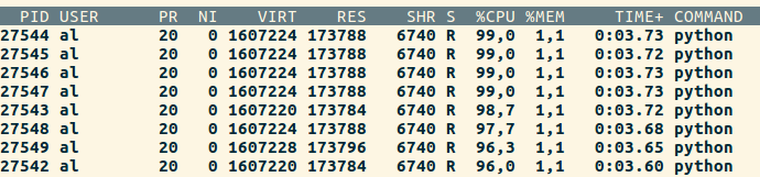
As you can see, it is now much faster because it spreads the work over all the available CPU cores.
Don't hesitate to use a system monitoring tool such as the top command to observe by yourself how xarray spawns a Python process for each of your CPU cores:
That's it for today! Thank you for reading and don't forget that you can always contact us if you need help to bring weather data into your own projects.